
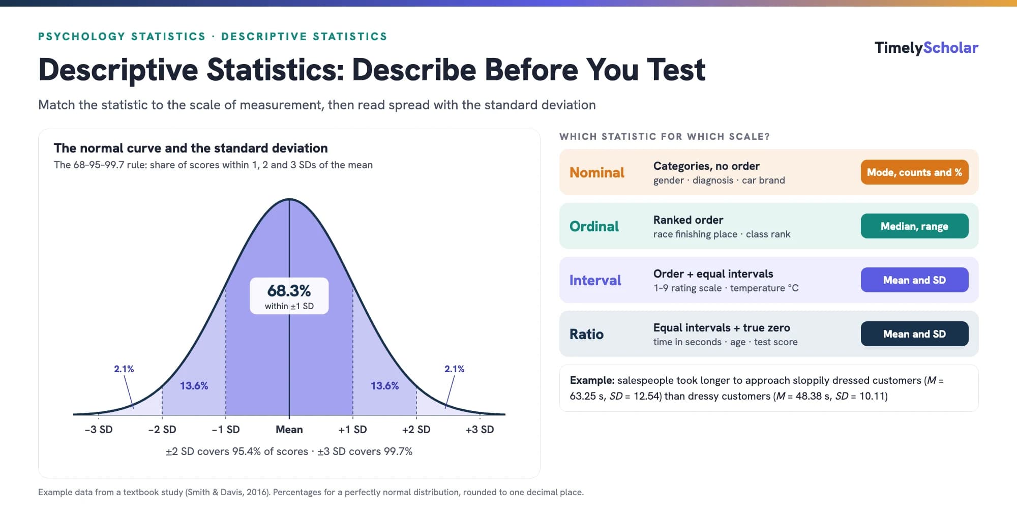
Descriptive statistics summarise a data set without testing hypotheses. They cover three things: the scale of measurement of each variable (nominal, ordinal, interval or ratio), its central tendency (mode, median or mean) and its variability (range, variance and standard deviation). Choose the statistic to fit the scale: counts and percentages for nominal variables such as gender, the median for ordinal variables, and the mean and standard deviation for interval and ratio variables such as age or reaction time. In SPSS, use Analyze > Compare Means > Means for group means, Descriptives for whole-sample means, and Frequencies for categories. In APA style, report them as, for example, M = 48.38, SD = 10.11.
Working on a psychology methods assignment or lab report? Get one-to-one support from a specialist. Get a free quote →
What are descriptive statistics?
Descriptive statistics do exactly what the name suggests: they describe your data. A mean, a percentage or a standard deviation condenses a column of raw numbers into a few values that a reader can take in at a glance (Kaur et al., 2018). Every quantitative report uses them twice: in the Method section, to describe the participants, and in the Results, to describe the outcome in each condition before any significance tests.
| Descriptive statistics | Inferential statistics | |
|---|---|---|
| Purpose | Summarise the sample you have | Draw conclusions about a wider population |
| Examples | Mean, median, mode, SD, range, counts, percentages | t-test, ANOVA, chi-square, correlation, regression |
| Answers | What do the data look like? | Is the difference or relationship bigger than chance? |
| Uses probability (p-values)? | No | Yes |
Inferential tests build on descriptive ones: an independent-samples t-test or a one-way ANOVA tells you whether group means differ, but it is the descriptive means and standard deviations that tell you which group scored higher and by how much. That is why APA reporting standards ask for descriptive statistics for every group and every key variable (Appelbaum et al., 2018).
Scales of measurement: nominal, ordinal, interval and ratio
The four scales of measurement, first set out by Stevens (1946), describe what the numbers in a variable mean. The scale decides which descriptive statistics, and later which tests, make sense, so settle it when you write each variable's operational definition.
| Scale | What it has | Psychology examples | Best descriptive statistics |
|---|---|---|---|
| Nominal | Categories with no order | Gender, diagnosis, yes/no answers, car brand | Counts (frequencies), percentages, mode |
| Ordinal | Categories in a ranked order, but unequal or unknown gaps | Finishing place in a race, class rank, food preference ranking | Median, range, percentiles |
| Interval | Order and equal intervals, but no true zero | A 1–9 rating scale, temperature in °C | Mean, standard deviation |
| Ratio | Order, equal intervals and a true zero | Reaction time, age, number of correct answers | Mean, standard deviation |
Two examples make the differences concrete. In a race, first, second and third place are ordinal: you know the order, but the first three runners might finish seconds apart and the fourth minutes behind. Time to finish, by contrast, is ratio: the gap between 10 and 20 seconds equals the gap between 50 and 60, and zero means no time at all.
Measures of central tendency: mean, median and mode
A measure of central tendency is a single number that represents the centre of a set of scores. Take the scores 12, 15, 15, 17, 17, 18, 20:
- Mode: the most frequent score. Here both 15 and 17 appear twice, so the set is bimodal. The mode is the only measure of central tendency that works for nominal data: if six participants are man, man, man, woman, woman, man, the modal category is men (4 of 6).
- Median: the middle score once the scores are put in order. With seven scores, the median is the fourth, 17. With an even number of scores, average the middle two: for 12, 15, 15, 17, 18, 20 the median is (15 + 17) / 2 = 16. Use it for ordinal, interval and ratio data.
- Mean: the arithmetic average. Add the scores and divide by how many there are: 114 / 7 = 16.29. Use it for interval and ratio data.
The mean uses every score, which makes it the most informative measure but also the most sensitive to extreme values. The median is robust: replace the 20 with 15,000, and the mean jumps to over 2,000 while the median stays at 17. For skewed variables such as income or reaction times with a few very slow responses, report the median as well, or instead (Mishra et al., 2019). Leys et al. (2013) make the same argument for detecting outliers, recommending the median absolute deviation over rules based on the mean and SD.
Measures of variability: range, variance and standard deviation
Two groups can share a mean but differ hugely in how spread out the scores are. Measures of variability capture that spread.
- Range: highest score minus lowest score. For 12, 15, 15, 17, 17, 18, 20, the range is 20 − 12 = 8. It is easy to calculate but depends entirely on the two most extreme scores, so a single outlier can inflate it enormously.
- Variance: the average squared distance of the scores from the mean. In a sample, the squared distances are added and divided by n − 1 rather than n, which SPSS does automatically.
- Standard deviation (SD): the square root of the variance. It is back in the original units (seconds, points, years), which is why the SD rather than the variance is what you report.
Dressy-condition approach times: 37, 38, 44, 47, 49, 49, 54, 69 seconds. Mean = 387 / 8 = 48.375.
Deviations from the mean: −11.38, −10.38, −4.38, −1.38, 0.63, 0.63, 5.63, 20.63.
Sum of the squared deviations = 715.88. Variance = 715.88 / (8 − 1) = 102.27.
SD = √102.27 = 10.11 seconds.
The standard deviation and the normal curve (the 68–95–99.7 rule)
When scores follow a normal (bell-shaped) distribution, the standard deviation tells you where most of them lie:
- About 68% of scores fall within 1 SD of the mean (34.1% on each side).
- About 95% fall within 2 SDs (adding 13.6% on each side).
- About 99.7% fall within 3 SDs (adding a further 2.1% on each side).
Imagine a sample with a mean age of 24. If the SD is 3 years, about 68% of participants are between 21 and 27: a tightly clustered group of young adults. If the SD is 10 years, the same 68% span 14 to 34, a much more varied sample. Reporting the SD alongside the mean lets readers picture the spread without seeing the raw data.
The rule is exact only for a normal distribution. Small samples and skewed variables can depart from it considerably, so check a histogram before relying on it (Mishra et al., 2019).
Worked example: approach times for dressy and sloppy customers
This example comes from a classic textbook study (Smith & Davis, 2016). Salespeople were randomly assigned to see a customer in dressy or sloppy clothes, and the researchers timed how many seconds passed before the salesperson approached. Clothing is the independent variable, time is the dependent variable (a ratio scale), and there are eight salespeople per condition (N = 16).
| Statistic | Dressy | Sloppy | All 16 |
|---|---|---|---|
| Scores | 37, 38, 44, 47, 49, 49, 54, 69 | 50, 46, 62, 52, 74, 69, 77, 76 | |
| Sum (Σ) | 387 | 506 | 893 |
| Mean | 48.38 | 63.25 | 55.81 |
| Median | 48.00 | 65.50 | 51.00 |
| Mode | 49 | None (every score occurs once) | 49 and 69 |
| Standard deviation | 10.11 | 12.54 | 13.42 |
| Range (min–max) | 32 (37–69) | 31 (46–77) | 40 (37–77) |
Notice the median for the sloppy group. The scores must be sorted first (46, 50, 52, 62, 69, 74, 76, 77), so the two middle scores are 62 and 69, and the median is 65.5. Averaging the fourth and fifth scores in the order they were recorded (52 and 74) would give the wrong answer, a common slip.
Using the SD, about 68% of dressy-condition salespeople would be expected to approach within 38.3 to 58.5 seconds (48.38 ± 10.11) and about 68% of sloppy-condition salespeople within 50.7 to 75.8 seconds (63.25 ± 12.54), if the times were normally distributed. With only eight scores per group, treat those ranges as a rough guide.
Descriptive statistics in SPSS, method 1: Means (by group)
SPSS offers three procedures for descriptive statistics, and each suits a different job. Use Means when you want the mean and SD of an outcome separately for each condition, which is what you need in a Results section.
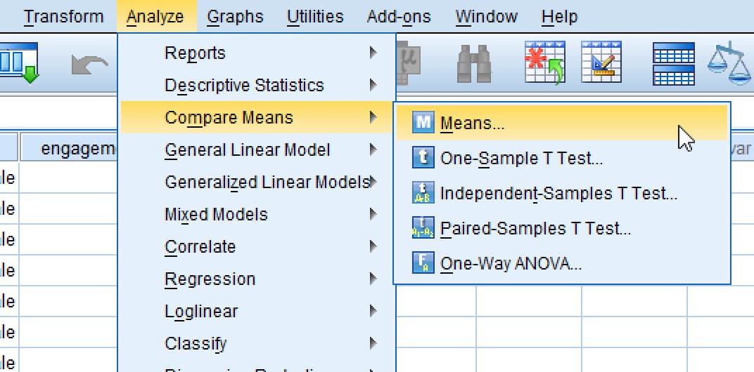
- Choose Analyze > Compare Means > Means.
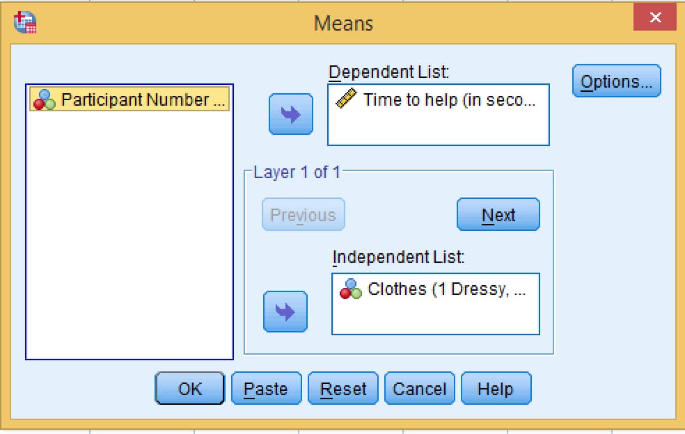
- Move the outcome (Time to help) into the Dependent List and the grouping variable (Clothes) into the Independent List.
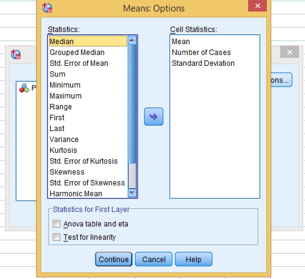
- Click Options. Mean, Number of Cases and Standard Deviation are selected by default; add Median, Minimum and Maximum if you want them. Click Continue, then OK.
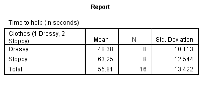
In APA style: salespeople took longer to approach customers in sloppy clothes (M = 63.25 s, SD = 12.54) than customers in dressy clothes (M = 48.38 s, SD = 10.11). Whether that difference is significant is a question for an inferential test.
Method 2: Descriptives (whole sample)
Use Descriptives for a quick summary of continuous variables across the whole sample, such as participants' age. It has no box for a grouping variable, so it cannot split results by condition.
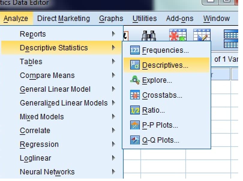
- Choose Analyze > Descriptive Statistics > Descriptives.
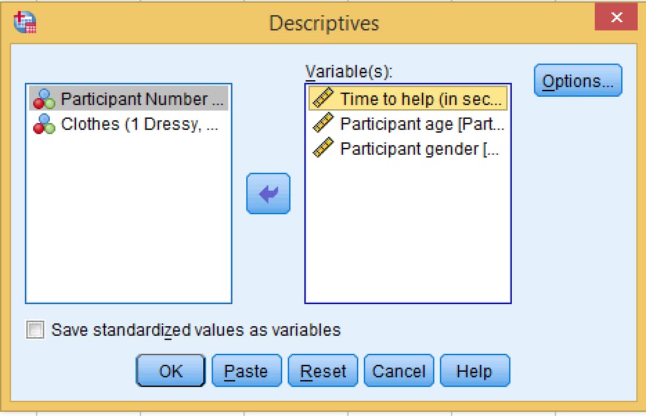
- Move the variables into the Variable(s) box.
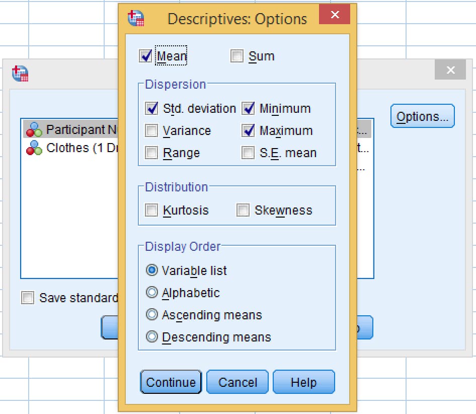
- Click Options and tick Mean, Std. deviation, Minimum and Maximum. Click Continue, then OK.
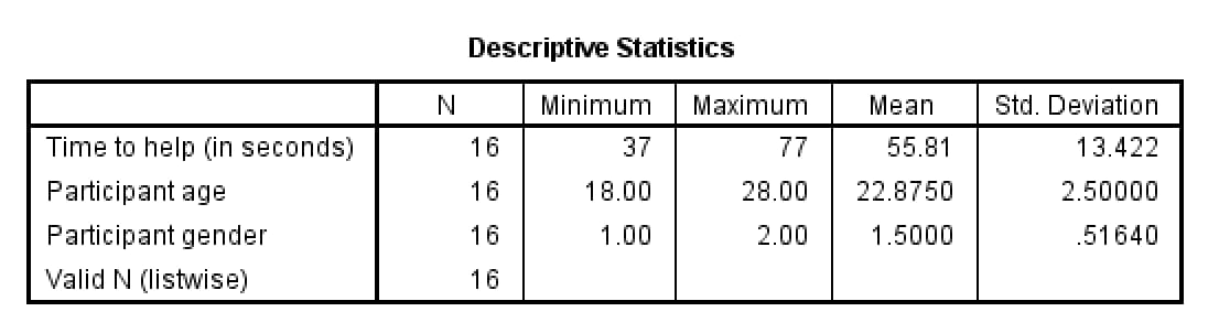
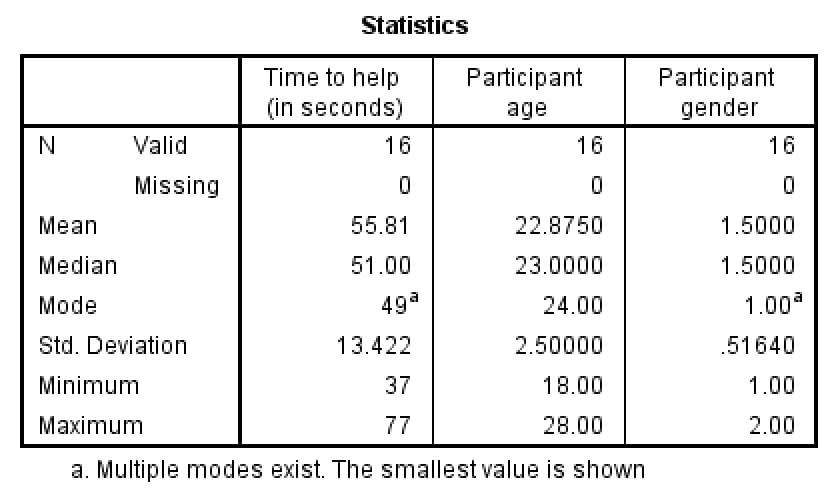
The age row gives everything you need: participants ranged in age from 18 to 28 years (M = 22.88, SD = 2.50). The time-to-help row matches the Total row from the Means procedure (M = 55.81, SD = 13.42), but without the split by condition. The gender row shows why the scale matters: a "mean gender" of 1.50 is meaningless because gender is nominal. For categories, use Frequencies.
Method 3: Frequencies (categories and demographics)
Frequencies counts how many participants fall into each category, which makes it the right procedure for nominal variables such as gender and ethnicity, and the best single procedure for writing a Participants section. It can also give the mean, median, mode, SD and range for continuous variables.
- Choose Analyze > Descriptive Statistics > Frequencies.
- Move your demographic and outcome variables into Variable(s) and keep Display frequency tables ticked.
- Click Statistics and tick Mean, Median and Mode under Central Tendency, and Std. deviation, Minimum and Maximum under Dispersion. Click Continue, then OK.
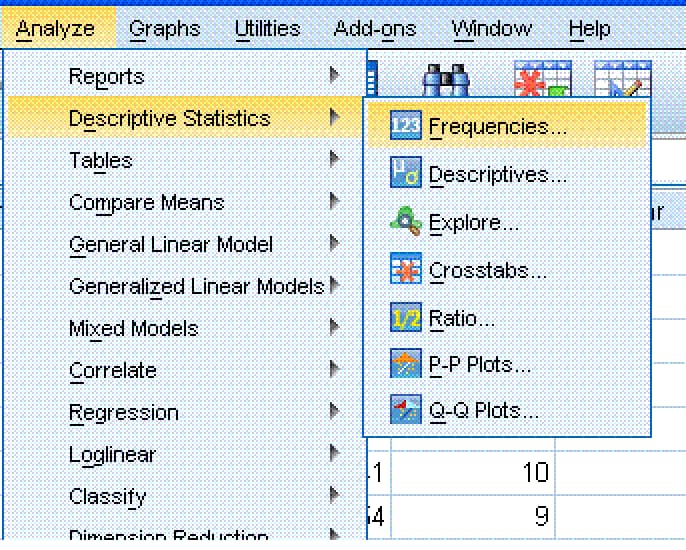
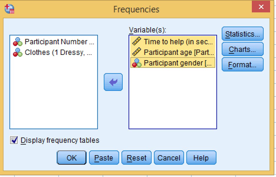
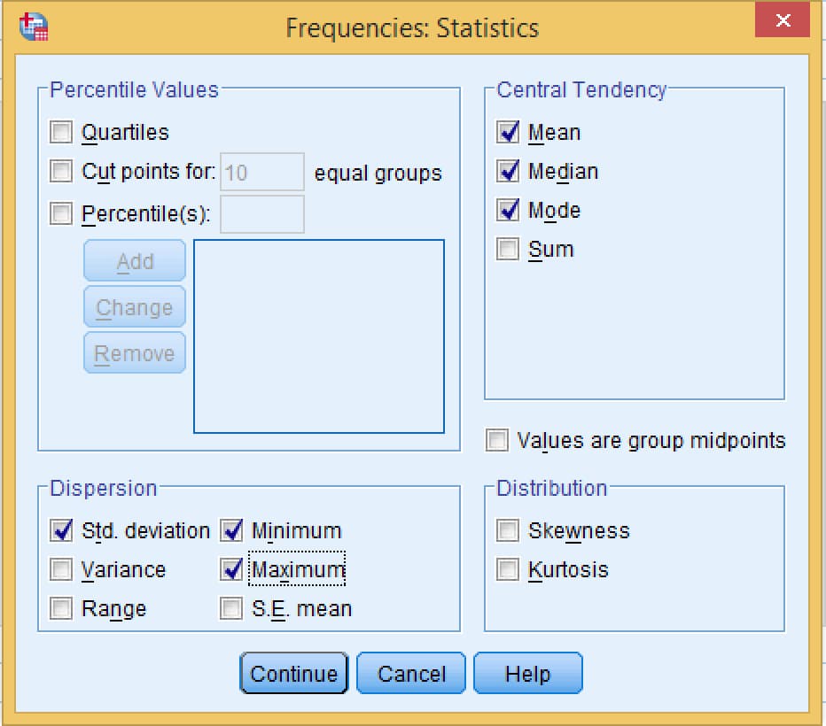
The Statistics table summarises every variable at once, including the median and mode that Descriptives does not give. Note the Missing row: it shows how many participants skipped each question.
Reading a frequency table
Each category gets its own row with four columns: Frequency (the count), Percent (of everyone in the data set, including those with missing answers), Valid Percent (of those who answered) and Cumulative Percent. In this version of the data, two participants did not report their gender:
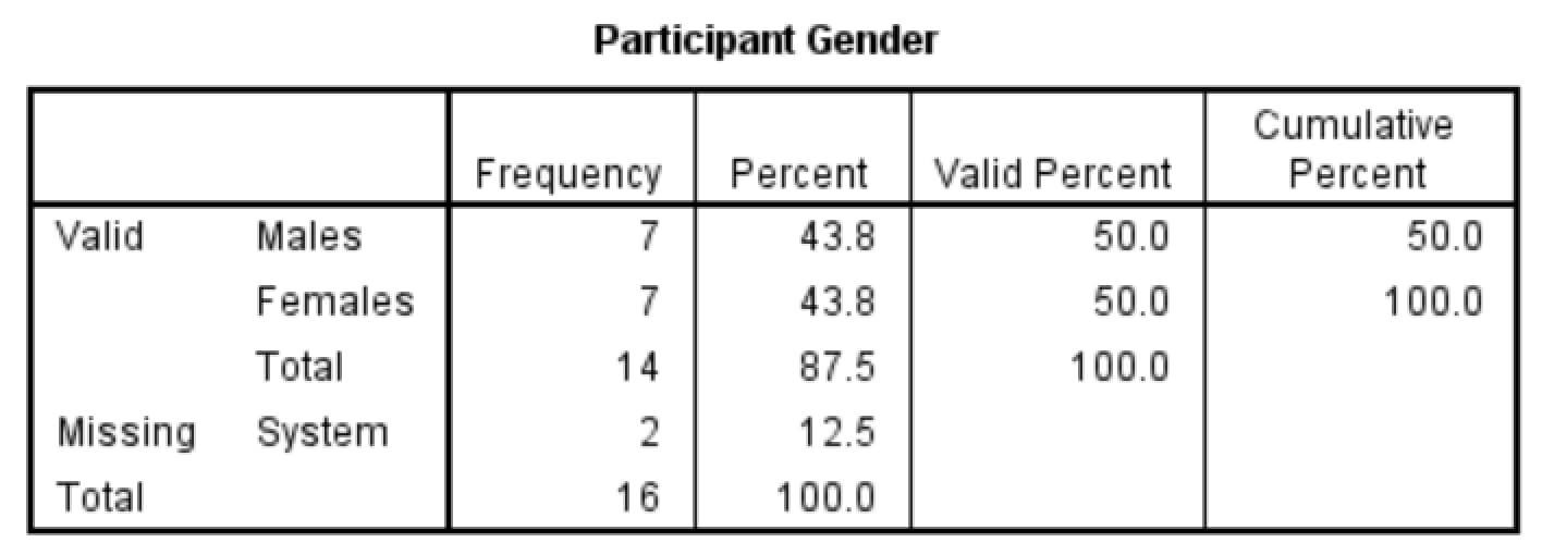
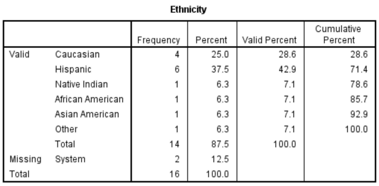
When you describe the whole sample, report the Percent column so that the percentages, including the missing group, add up to 100%. The same logic applies to ethnicity:
SPSS also prints frequency tables for continuous variables such as age and time, listing every distinct value. These are rarely useful in a report; summarise those variables with the mean and SD instead.
Means vs Descriptives vs Frequencies: which SPSS procedure?
| Procedure | Menu | Best for | Limitation |
|---|---|---|---|
| Means | Analyze > Compare Means > Means | Mean and SD of an outcome for each condition | Not for categorical variables |
| Descriptives | Analyze > Descriptive Statistics > Descriptives | Quick whole-sample summary of continuous variables (e.g. age) | No median or mode; no split by group |
| Frequencies | Analyze > Descriptive Statistics > Frequencies | Counts and percentages for categories; full summary for the Participants section | Long output; frequency tables for continuous variables are rarely useful |
Inferential procedures also produce descriptive statistics: the t-test, ANOVA and Crosstabs dialogs each have options that print means, standard deviations or counts for each group, as shown in our guides to the one-way ANOVA and the chi-square test.
How to report descriptive statistics in APA 7
APA style uses italic symbols: M for the mean, SD for the standard deviation, Mdn for the median, N for the whole sample and n for a subgroup, with two decimal places for most statistics (American Psychological Association, 2020). Our guide to reporting statistics in APA 7 covers the formatting rules in detail.
Describing participants (Method section)
JARS asks authors to describe the sample's major demographic characteristics, including age, gender and race or ethnicity and to report missing data (Appelbaum et al., 2018). Describe categories as participants identified themselves, and use current bias-free terms: for example, APA guidance recommends "White" rather than "Caucasian" (American Psychological Association, 2023).
Sixteen participants (8 men, 8 women) took part. They ranged in age from 18 to 28 years (M = 22.88, SD = 2.50).
Sixteen participants took part: 7 men (43.8%), 7 women (43.8%) and 2 who did not report their gender (12.5%). Participants ranged in age from 18 to 28 years (M = 22.88, SD = 2.50). Six identified as Hispanic (37.5%), four as White (25.0%), and one each (6.3%) as African American, Asian American, Native American or another ethnicity; two did not report their ethnicity (12.5%).
Describing outcomes (Results section)
Salespeople took longer to approach customers wearing sloppy clothes (M = 63.25 s, SD = 12.54) than customers wearing dressy clothes (M = 48.38 s, SD = 10.11).
When you have more than a few groups or variables, put the descriptive statistics in a table instead of the text. Our free Table 1 generator builds an APA-formatted participant characteristics table from your data.
Common mistakes with descriptive statistics
- Reporting a mean or SD for a nominal variable, such as a "mean gender" of 1.50.
- Finding the median without sorting the scores first.
- Reporting only the mean. Always pair it with the SD (or the median with the range or interquartile range).
- Using the mean for heavily skewed data without also reporting the median.
- Reporting Valid Percent when describing the whole sample, which hides participants who skipped a question.
- Inconsistent numbers between the text, tables and output; copy values carefully and round consistently to two decimal places.
- Using outdated or imposed demographic labels instead of the categories participants chose.
Getting help with statistics in your research methods course
If you would like a specialist to check your SPSS output, help you choose the right descriptive statistics or give feedback on your Participants and Results sections, see our psychology research methods and statistics support. We explain each step so you can apply it confidently in your own work.
Frequently asked questions
What are descriptive statistics?
Statistics that summarise a data set: its scale of measurement, central tendency (mean, median, mode) and variability (range, variance, standard deviation), plus counts and percentages for categories. They describe the sample without testing hypotheses.
What is the difference between descriptive and inferential statistics?
Descriptive statistics summarise the data you collected. Inferential statistics, such as t-tests and ANOVA, use the data to draw conclusions about a wider population and produce p values.
What are the four scales of measurement?
Nominal (categories with no order), ordinal (ranked categories), interval (equal intervals but no true zero) and ratio (equal intervals and a true zero).
When should I use the mean, median or mode?
Use the mode for nominal data, the median for ordinal data or skewed interval and ratio data, and the mean for interval and ratio data that are roughly symmetrical.
What does the standard deviation tell you?
How spread out the scores are around the mean. In a normal distribution, about 68% of scores fall within one SD of the mean, 95% within two and 99.7% within three.
How do I get descriptive statistics in SPSS?
Use Analyze > Compare Means > Means for means by group, Analyze > Descriptive Statistics > Descriptives for whole-sample means and SDs, and Analyze > Descriptive Statistics > Frequencies for counts, percentages, medians and modes.
How do I report descriptive statistics in APA 7?
Use italic symbols with two decimal places, for example M = 48.38, SD = 10.11, and report counts with percentages for categories, for example 7 men (43.8%). Put larger sets of statistics in a table.
How do I report demographics with missing data?
Report the count and the Percent column (not Valid Percent) for each category, including the number who did not answer, so that the percentages add up to 100%.
Sources
- Field A. Discovering Statistics Using IBM SPSS Statistics. 6th ed. London: Sage; 2024
- Mishra P, Pandey CM, Singh U, Gupta A, Sahu C, Keshri A. Descriptive statistics and normality tests for statistical data. Ann Card Anaesth 2019;22(1):67-72
- American Psychological Association. Inclusive Language Guide. 2nd ed. Washington, DC: American Psychological Association; 2023
- American Psychological Association. Publication Manual of the American Psychological Association. 7th ed. Washington, DC: American Psychological Association; 2020
- Appelbaum M, Cooper H, Kline RB, et al. Journal article reporting standards for quantitative research in psychology: the APA Publications and Communications Board task force report. Am Psychol 2018;73:3-25
- Kaur P, Stoltzfus J, Yellapu V. Descriptive statistics. Int J Acad Med 2018;4(1):60-63
- Leys C, Ley C, Klein O, Bernard P, Licata L. Detecting outliers: do not use standard deviation around the mean, use absolute deviation around the median. J Exp Soc Psychol 2013;49(4):764-766
- Stevens SS. On the theory of scales of measurement. Science 1946;103(2684):677-680
- Smith RA, Davis SF. The Psychologist as Detective: An Introduction to Conducting Research in Psychology. Updated ed. Boston, MA: Pearson; 2016

Michael has 6 years of experience in health research, nursing, public health, the social sciences, and qualitative evidence synthesis. He leads or supports projects that organize and interpret qualitative findings while preserving the context of the original studies. Areas of expertise Qualitative evidence…