
![Independent-samples t-test example: dot plot of time to approach dressy (M = 48.38, SD = 10.11) and sloppy (M = 63.25, SD = 12.54) customers with 95% confidence intervals, and the results t(14) = -2.61, p = .021, Welch t(13.40) = -2.61, mean difference -14.88 seconds [-27.09, -2.66], Cohen's d = 1.31](/_next/image?url=%2Fimages%2Findependent-samples-t-test-spss-example-cohens-d.webp&w=3840&q=75)
An independent-samples t-test compares the means of two separate groups on a continuous outcome, such as reaction time or a 1–9 rating, to see whether the difference is larger than chance. In SPSS, run it from Analyze > Compare Means > Independent-Samples T Test: put the outcome in Test Variable(s) and the group variable in Grouping Variable, then define the two groups. Check Levene's test to choose the row to read (or simply use Welch's "equal variances not assumed" row), and report it in APA style as t(df) = value, p = value, with Cohen's d and each group's mean and standard deviation, for example: t(14) = 2.61, p = .021, d = 1.31.
Working on a psychology methods assignment or lab report? Get one-to-one support from a specialist. Get a free quote →
What is an independent-samples t-test?
The independent-samples t-test (also called the two-sample or between-subjects t-test) asks whether two groups that contain different people differ, on average, on a continuous measure. Typical psychology examples include comparing anxiety scores for a treatment and a control group (or two intact classes, as in a quasi-experiment), or recall for participants who studied with or without music (Field, 2024).
The test needs two pieces of information. The descriptive statistics, the mean and standard deviation of each group, show the size and direction of the difference. The t statistic is inferential: it divides the difference between the means by its standard error, so it grows as the difference gets bigger and as the scores within each group become less variable or more numerous. The larger t is, the smaller the p-value, and if p < .05, the difference is statistically significant.
A t-test result is written in a standard form: t(14) = 2.61, p = .021. The t says which test was used, 14 is the degrees of freedom, 2.61 is the value of the statistic, and p is the probability of a difference at least this large if the groups did not really differ.
Types of t-test: independent, paired and one-sample
| Test | Compares | Example | SPSS menu |
|---|---|---|---|
| Independent-samples t-test | Means of two separate groups | Treatment group vs control group | Compare Means > Independent-Samples T Test |
| Paired-samples t-test | Two means from the same people (or matched pairs) | Anxiety before vs after therapy | Compare Means > Paired-Samples T Test |
| One-sample t-test | One mean against a known value | Class IQ vs the population mean of 100 | Compare Means > One-Sample T Test |
If you have two independent variables, use a two-way factorial ANOVA. If you have three or more groups, use a one-way ANOVA instead of several t-tests, which would inflate the false-positive rate. If your outcome is a category (yes/no, guilty/not guilty), a t-test is not possible because there is no mean to compare; use a chi-square test. For a full decision guide, see which statistical test should I use.
Independent t-test assumptions
| Assumption | How to check | If violated |
|---|---|---|
| Continuous dependent variable (interval or ratio) | How was it measured? A rating scale, a time, a score | Use a chi-square test for categories, or Mann-Whitney U for ranks |
| Two independent groups: each person in one group only | Check the design | Use a paired-samples t-test |
| Roughly normal scores in each group | Histograms or Q-Q plots per group | Usually fine with moderate samples; with small, skewed samples, consider Mann-Whitney U |
| Equal variances (homogeneity of variance) | Levene's test; compare the two SDs | Use Welch's t-test (the "equal variances not assumed" row) |
| No extreme outliers | Box plots | Check for errors; report results with and without genuine outliers |
The t-test copes well with moderate departures from normality, especially when the groups are similar in size (Blanca et al., 2017; Kim, 2015). Unequal variances matter more. Because Levene's test itself can miss real differences in small samples and overreact in large ones, Delacre et al. (2017) recommend reporting Welch's t-test by default: it is almost as powerful as Student's t-test when variances are equal and much more accurate when they are not. Ruxton (2006) made the same case, noting that Welch's test is also often a better choice than switching to the Mann-Whitney U test.
Hypotheses: one-tailed vs two-tailed t-tests
The null hypothesis says the two population means are equal; the alternative hypothesis says they differ. A two-tailed test, the default in SPSS and in most journals, looks for a difference in either direction. A one-tailed test looks in only one direction and halves the p-value: here, a one-tailed test would give p = .010 instead of .021.
Use a one-tailed test only if you stated the direction before collecting data and would treat a result in the other direction exactly like no difference. Choosing a one-tailed test after seeing the data, to push p below .05, is not legitimate. When in doubt, report the two-tailed result.
Worked example: does a customer's clothing change how fast they are served?
This example comes from a classic textbook study (Smith & Davis, 2016). Salespeople were randomly assigned to see a customer in dressy or sloppy clothes, and the researchers timed how many seconds passed before the salesperson approached. Clothing is the independent variable (two groups), time is the continuous dependent variable, and there are eight salespeople per group (N = 16). The prediction: dressy customers will be approached faster.
| Dressy | Sloppy | |
|---|---|---|
| Scores | 37, 38, 44, 47, 49, 49, 54, 69 | 50, 46, 62, 52, 74, 69, 77, 76 |
| Sum (Σ) | 387 | 506 |
| Mean (M) | 48.38 | 63.25 |
| Standard deviation (SD) | 10.11 | 12.54 |
The means support the prediction: salespeople took about 15 seconds longer to approach the sloppily dressed customer. Whether a difference that size could easily arise by chance in groups of eight is what the t-test answers. For how the means and standard deviations are calculated, see our guide to descriptive statistics in SPSS.
How to run an independent-samples t-test in SPSS
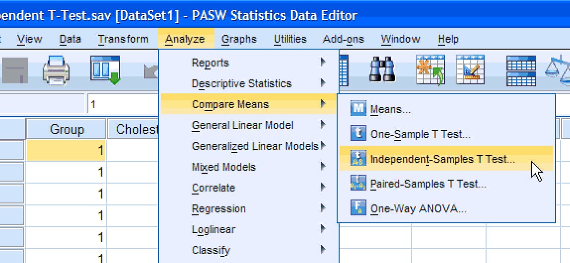
Enter one row per participant: a grouping variable (Clothes: 1 = dressy, 2 = sloppy, with value labels) and the outcome (time in seconds). Then:
- Choose Analyze > Compare Means > Independent-Samples T Test.
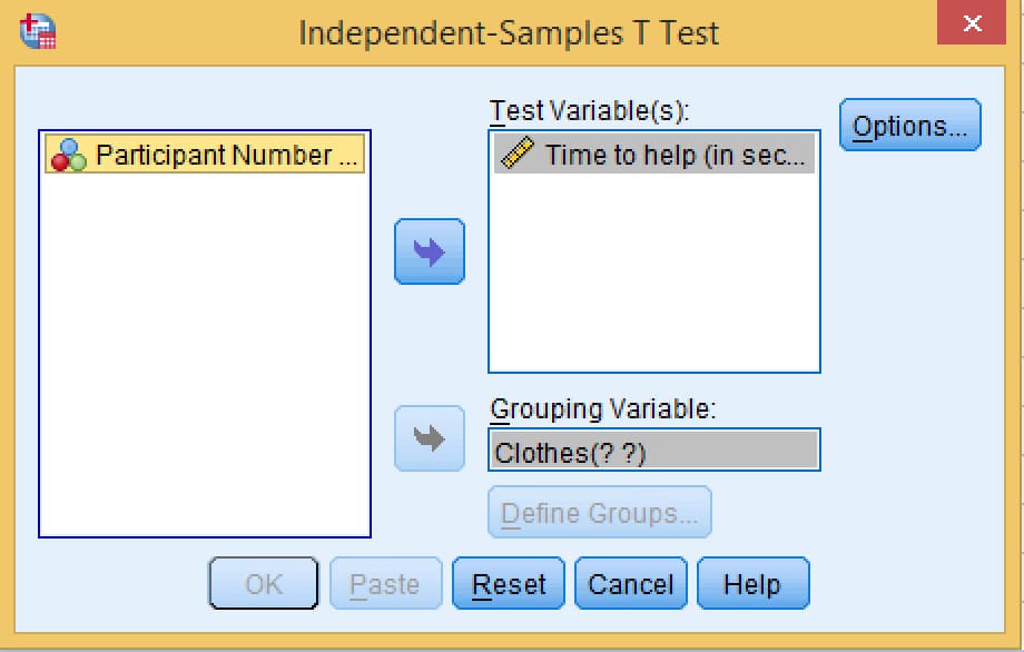
- Move the outcome (Time to help) into Test Variable(s) and the group variable (Clothes) into Grouping Variable. SPSS calls the dependent variable the test variable and the independent variable the grouping variable.
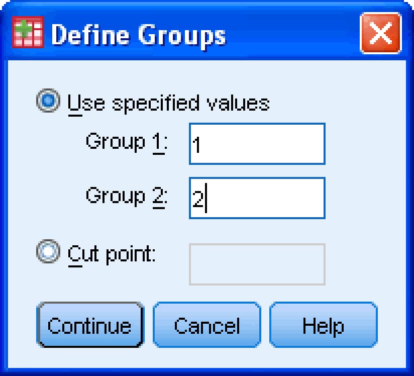
- Click Define Groups and enter the codes of the two groups you want to compare: 1 in Group 1 and 2 in Group 2. If your variable has more codes (say 3 = casual), you can compare any two of them, such as 1 and 3. Click Continue.
- In recent SPSS versions, keep Estimate effect sizes ticked to get Cohen's d automatically. Click OK.
How to interpret independent t-test output in SPSS
1. Group Statistics
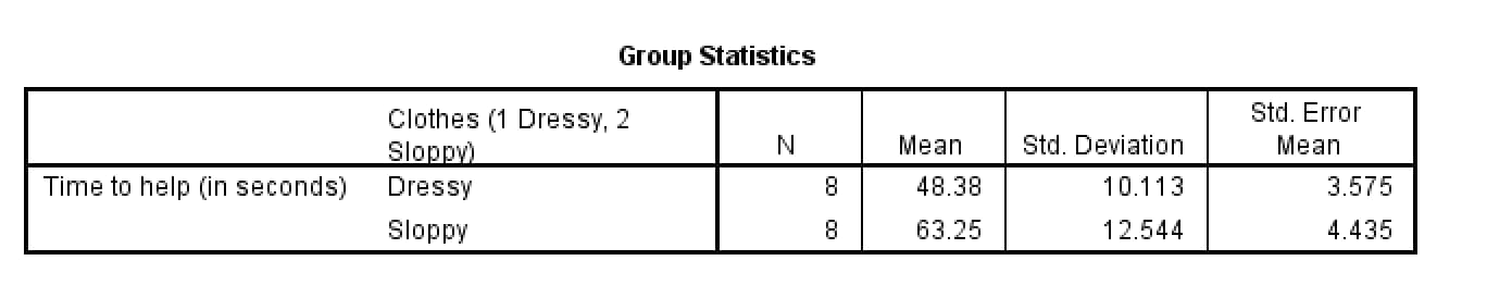
The first table gives N, the mean, standard deviation and standard error of the mean for each group. Dressy: M = 48.38, SD = 10.11; sloppy: M = 63.25, SD = 12.54. You will need these for the write-up.
2. Independent Samples Test
The second table contains Levene's test and two rows of t-test results. In full, it looks like this:
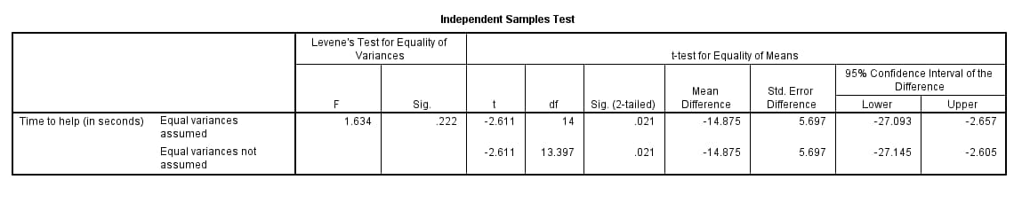
Read it in three steps:
- Levene's test (F and Sig.) tests whether the two variances are equal. Here F = 1.63, p = .222. Because p > .05, the variances are not significantly different, so the Equal variances assumed row is the traditional choice. If Levene's p were below .05, you would read the Equal variances not assumed (Welch) row instead.
- t, df and Sig. (2-tailed) are the test itself: t(14) = −2.61, p = .021. The Welch row gives almost the same result, t(13.40) = −2.61, p = .021; its decimal degrees of freedom are normal.
- Mean Difference and the 95% Confidence Interval of the Difference show the size of the effect in the original units: dressy minus sloppy = −14.88 seconds, 95% CI [−27.09, −2.66]. Because the interval does not include 0, the difference is significant at the .05 level.
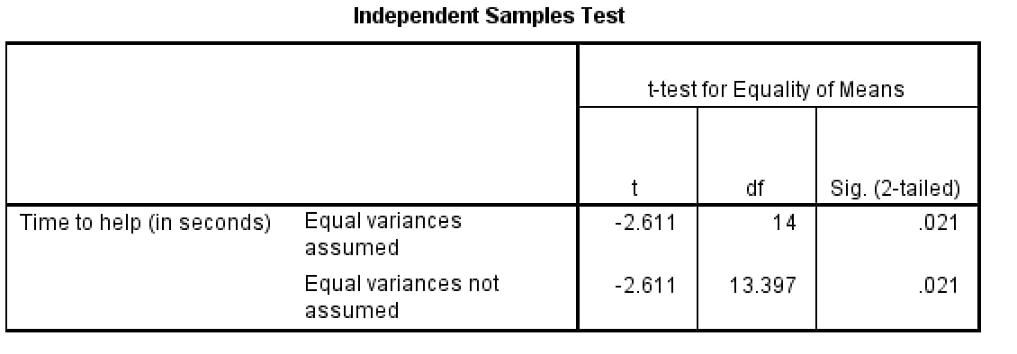
Why is t negative?
SPSS subtracts Group 2 from Group 1 (dressy minus sloppy). Because the dressy mean is lower, t and the mean difference are negative. The sign only reflects the order in which you defined the groups; swapping them would give t = 2.61. Report the absolute value and describe the direction in words.
Effect size for a t-test: Cohen's d
A significant p-value tells you the difference is unlikely to be chance; Cohen's d tells you how big it is, in standard deviation units. It is the difference between the means divided by the pooled standard deviation (Lakens, 2013):
Pooled SD = √[((8 − 1) × 10.11² + (8 − 1) × 12.54²) / 14] = 11.39.
d = (63.25 − 48.38) / 11.39 = 1.31.
Cohen's (1992) benchmarks are 0.20 small, 0.50 medium and 0.80 large, so 1.31 is a large effect: the sloppy group's average was more than one standard deviation slower. Two cautions: with only eight people per group the estimate is imprecise (its 95% confidence interval runs from roughly 0.23 to 2.38), and d slightly overestimates the population effect in small samples. Hedges' g corrects that bias; here g = 1.23. Convert between effect sizes with our effect size calculator.
How to report an independent t-test in APA 7
Report the means and standard deviations of both groups, t with its degrees of freedom, the exact p value, an effect size and ideally the confidence interval for the difference (American Psychological Association, 2020; Appelbaum et al., 2018). Italicise the statistical symbols and drop the leading zero from p. Our guide to reporting statistics in APA 7 covers the formatting rules.
An independent-samples t-test compared the time salespeople took to approach customers in dressy and sloppy clothing. Salespeople approached customers in dressy clothing (M = 48.38 s, SD = 10.11) significantly faster than customers in sloppy clothing (M = 63.25 s, SD = 12.54), t(14) = 2.61, p = .021, d = 1.31, 95% CI for the difference [2.66, 27.09].
Salespeople approached customers in dressy clothing faster than customers in sloppy clothing, Welch's t(13.40) = 2.61, p = .021, d = 1.31.
For a non-significant result, use the same format, for example t(58) = 1.12, p = .267, d = 0.29, and say that the groups did not differ significantly rather than that they were "the same".
When assumptions are violated: Welch's t-test and Mann-Whitney U
- Unequal variances: read the "Equal variances not assumed" row (Welch's t-test). Many researchers now report this row by default (Delacre et al., 2017).
- Ordinal outcome or small, heavily skewed samples: use the Mann-Whitney U test (Analyze > Nonparametric Tests > Independent Samples), which compares ranks rather than means. Try it with our Mann-Whitney U calculator.
- The same people in both conditions: use the paired-samples t-test instead.
Degrees of freedom for an independent t-test
For Student's independent t-test, df = n₁ + n₂ − 2: here 8 + 8 − 2 = 14. Two degrees of freedom are lost because each group's mean is estimated from the data. Welch's t-test adjusts the degrees of freedom downwards when the variances differ, which is why its df is usually a decimal (13.40 here). Report the value SPSS gives, rounded to two decimal places.
Common t-test mistakes
- Swapping the boxes: the outcome belongs in Test Variable(s), the group variable in Grouping Variable.
- Forgetting to define the groups, which leaves Clothes(? ?) and a greyed-out OK button.
- Reading the wrong row of the Independent Samples Test table, or reporting Levene's F as the result.
- Running a t-test on three or more groups by comparing pairs; use ANOVA.
- Using an independent t-test for repeated measurements of the same people.
- Leaving out the means and SDs or the effect size.
- Writing p = .000. Report p < .001.
- Choosing a one-tailed test after seeing the results.
Getting help with t-tests in your statistics course
If you would like a specialist to check your SPSS setup, talk through your output or give feedback on your APA results section, see our psychology research methods and statistics support. We explain each step so you can apply it confidently in your own work.
Frequently asked questions
When should I use an independent-samples t-test?
When you compare the means of two separate groups of people on a continuous outcome, such as a treatment and a control group on anxiety scores.
What is the difference between an independent and a paired t-test?
An independent t-test compares two different groups of people. A paired t-test compares two measurements from the same people, or from matched pairs, such as scores before and after an intervention.
How do I interpret Levene's test in SPSS?
If Levene's Sig. value is above .05, the variances are similar and you can read the Equal variances assumed row. If it is below .05, read the Equal variances not assumed (Welch) row. Many researchers report the Welch row by default.
Why is my t value negative in SPSS?
SPSS subtracts the second group's mean from the first. A negative t only means Group 1 had the lower mean; report the absolute value and describe the direction in words.
How do I report an independent t-test in APA 7?
Give each group's mean and standard deviation and then t(df) = value, p = value, and an effect size, for example t(14) = 2.61, p = .021, d = 1.31, ideally with the 95% confidence interval for the difference.
How do you calculate Cohen's d for an independent t-test?
Divide the difference between the two means by the pooled standard deviation. Values of about 0.20, 0.50 and 0.80 are conventionally small, medium and large.
Should I use a one-tailed or two-tailed t-test?
Use a two-tailed test unless you predicted the direction of the difference before collecting data and would treat a difference in the other direction as no effect.
What are the degrees of freedom for an independent t-test?
For Student's t-test, df = n1 + n2 − 2. For Welch's t-test SPSS calculates an adjusted, usually decimal, value.
Sources
- Field A. Discovering Statistics Using IBM SPSS Statistics. 6th ed. London: Sage; 2024
- Delacre M, Lakens D, Leys C. Why psychologists should by default use Welch's t-test instead of Student's t-test. Int Rev Soc Psychol 2017;30(1):92-101
- American Psychological Association. Publication Manual of the American Psychological Association. 7th ed. Washington, DC: American Psychological Association; 2020
- Appelbaum M, Cooper H, Kline RB, et al. Journal article reporting standards for quantitative research in psychology: the APA Publications and Communications Board task force report. Am Psychol 2018;73:3-25
- Blanca MJ, Alarcón R, Arnau J, Bono R, Bendayan R. Non-normal data: is ANOVA still a valid option? Psicothema 2017;29(4):552-557
- Kim TK. T test as a parametric statistic. Korean J Anesthesiol 2015;68(6):540-546
- Lakens D. Calculating and reporting effect sizes to facilitate cumulative science: a practical primer for t-tests and ANOVAs. Front Psychol 2013;4:863
- Ruxton GD. The unequal variance t-test is an underused alternative to Student's t-test and the Mann-Whitney U test. Behav Ecol 2006;17(4):688-690
- Cohen J. A power primer. Psychol Bull 1992;112(1):155-159
- Smith RA, Davis SF. The Psychologist as Detective: An Introduction to Conducting Research in Psychology. Updated ed. Boston, MA: Pearson; 2016

Keith has 17 years of experience in experimental psychology and cognitive and behavioral research. He brings an experimental research perspective to projects that examine cognition, perception, and behavior. Areas of expertise Experimental and behavioral studies Quantitative research projects and data analysis…