
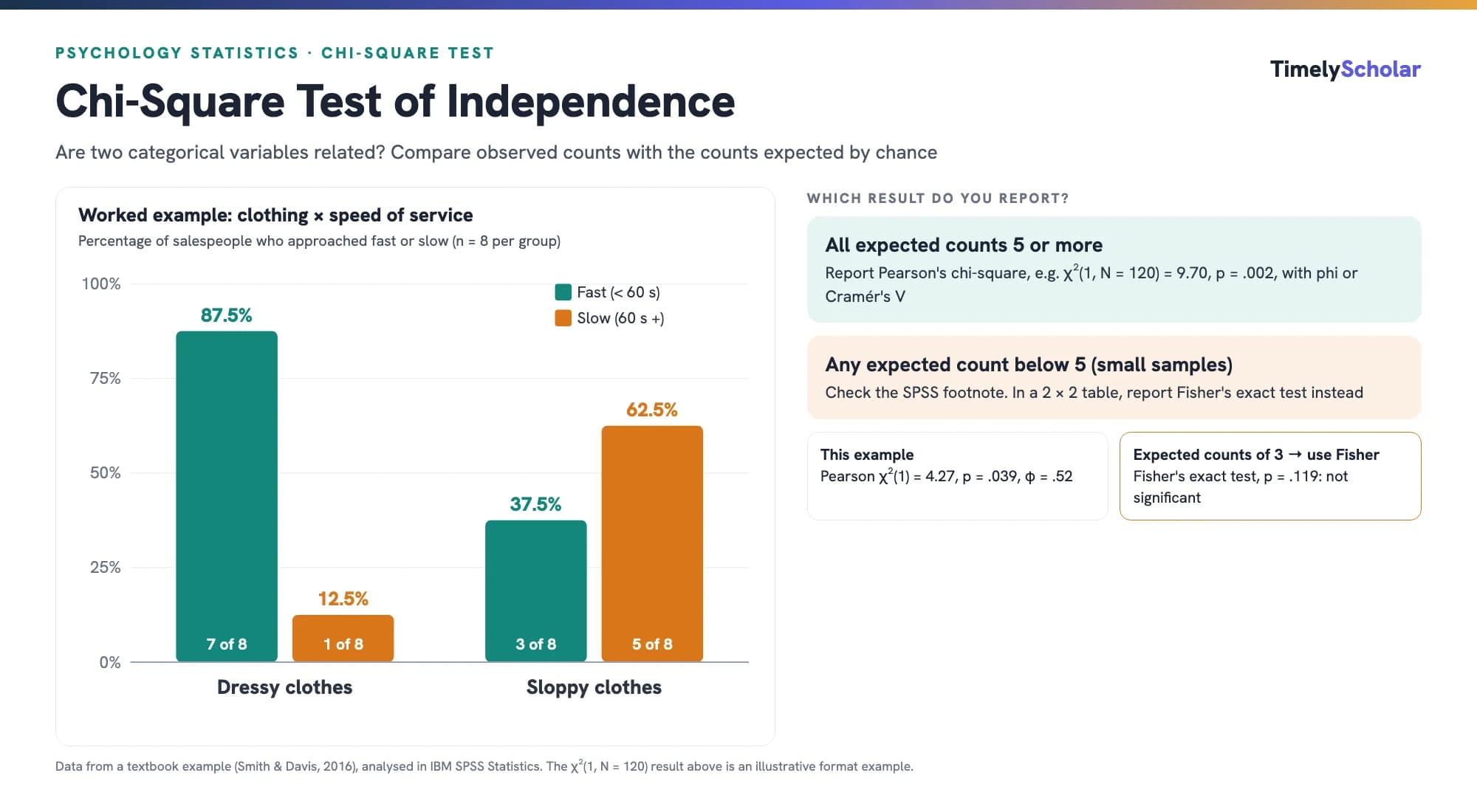
A chi-square (χ²) test of independence checks whether two categorical variables are related, by comparing the counts you observed in each cell of a contingency table with the counts you would expect if the variables were unrelated. In SPSS, run it with Analyze > Descriptive Statistics > Crosstabs, ticking Chi-square and Phi and Cramér's V under Statistics. Report it in APA style as χ²(df, N = sample size) = value, p = value, with phi or Cramér's V and the percentages in each group. The test assumes independent observations and adequate expected counts: if any expected count in a 2 × 2 table is below 5, report Fisher's exact test instead.
Working on a psychology methods assignment or lab report? Get one-to-one support from a specialist. Get a free quote →
What is a chi-square test?
Most tests students meet first, such as the t-test and ANOVA, compare means. They need an outcome measured on a scale: a rating from 1 to 9, a test score, a time in seconds. But many psychology outcomes are categories: guilty or not guilty, yes or no, which of four brands someone chose. A "mean verdict" makes no sense, so instead the chi-square test works with frequencies: how many cases fall into each category (McHugh, 2013).
Categorical variables come in two kinds (see our guide to scales of measurement and descriptive statistics for all four scales):
- Nominal: categories with no order, such as gender, diagnosis, or car brand (Honda, Toyota, Ford). None is higher or better than another.
- Ordinal: categories with a rank order but unknown distances between them, such as first, second and third place in a race. The chi-square test treats ordinal categories as if they were nominal, so it ignores the order.
The test asks a simple question: are the differences between the counts you observed and the counts you would expect by chance too large to be chance alone? The statistic adds up those differences across all the cells:
Goodness of fit vs test of independence
There are two common chi-square tests, and the difference is the number of variables.
| Goodness-of-fit test | Test of independence | |
|---|---|---|
| Variables | One categorical variable | Two categorical variables |
| Question | Do the counts match an expected distribution? | Are the two variables related? |
| Example | Are there more not-guilty-than-guilty verdicts than chance (50/50) would predict? | Does the juror's gender affect the verdict? |
| Degrees of freedom | Number of categories − 1 | (rows − 1) × (columns − 1) |
| SPSS menu | Analyze > Nonparametric Tests > Legacy Dialogs > Chi-square | Analyze > Descriptive Statistics > Crosstabs |
Two goodness-of-fit illustrations show how the test separates chance from a real pattern. If you sample 200 people and get 95 men and 105 women, the gap from a 50/50 split is easily explained by chance: χ²(1, N = 200) = 0.50, p = .480. If 60 of 100 jurors vote guilty and 40 not guilty, the imbalance is just large enough to be unlikely under a 50/50 expectation: χ²(1, N = 100) = 4.00, p = .046.
The rest of this guide focuses on the test of independence, which is the version most often used in psychology research methods courses. A related design, the test of homogeneity, uses the same calculation but samples each group separately; the arithmetic and SPSS steps are identical.
Chi-square assumptions (and when they are violated)
The chi-square test makes no assumption about a bell-shaped distribution, which is why it is often described as having few assumptions. It does have some, and the third causes the most mistakes (Kim, 2017; McHugh, 2013):
- Both variables are categorical, with mutually exclusive categories. If your outcome is a score, use a t-test or ANOVA instead.
- Observations are independent: each person contributes to one cell only. Before-and-after data from the same people need McNemar's test instead.
- Expected counts are large enough. The classic guideline, from Cochran (1954), is that no expected count should be below 1 and no more than 20% of cells should have expected counts below 5. In a 2 × 2 table, that means every expected count should be at least 5.
Expected counts are calculated, not observed: for each cell, multiply the row total by the column total and divide by the overall N. SPSS checks them for you and reports the result in a footnote under the Chi-Square Tests table, such as "2 cells (50.0%) have expected count less than 5". When the guideline is broken, the chi-square p-value can be misleading, and you have three options:
- Report Fisher's exact test, which SPSS prints automatically for 2 × 2 tables.
- For larger tables, use an exact test (the Exact button in Crosstabs, if your SPSS licence includes it) or combine categories where that makes theoretical sense.
- Collect more data, which is the best fix when you are still planning the study.
Worked example: does clothing affect how fast customers are served?
This example adapts a classic textbook study (Smith & Davis, 2016). Salespeople were randomly assigned to see a customer in dressy or sloppy clothes, and each salesperson's approach time was classified as fast (under 60 seconds) or slow (60 seconds or more). Clothing is the independent variable, speed of service is the categorical dependent variable, and there are eight salespeople per condition (N = 16).
| Clothing | Fast | Slow | Total |
|---|---|---|---|
| Dressy | 7 (5.0) | 1 (3.0) | 8 |
| Sloppy | 3 (5.0) | 5 (3.0) | 8 |
| Total | 10 | 6 | 16 |
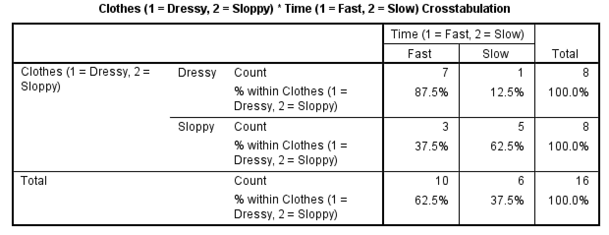
Seven of eight salespeople (87.5%) approached the dressy customer quickly, compared with three of eight (37.5%) for the sloppy customer. If clothing made no difference, you would expect the 10 fast responses to be split evenly, five per group: the expected count for dressy/fast is 8 × 10 / 16 = 5.0, and for dressy/slow it is 8 × 6 / 16 = 3.0. Plugging the four cells into the formula gives χ² = 0.80 + 1.33 + 0.80 + 1.33 = 4.27. The chart at the top of this guide shows the same pattern as a clustered bar chart.
Notice that the expected counts for the slow column are 3.0, below the threshold of 5. Keep that in mind; it changes what you report.
How to run a chi-square test in SPSS (Crosstabs)
Enter one row per participant, with a column for each variable (for example, Clothes: 1 = dressy, 2 = sloppy; Time: 1 = fast, 2 = slow) and value labels. The numbers are only codes; any two values would do. Then:
- Choose Analyze > Descriptive Statistics > Crosstabs.
- Move one variable into Row(s) and the other into Column(s). There is no right or wrong choice; putting the independent variable in the rows makes row percentages easy to read. Tick Display clustered bar charts.
- Click Statistics, tick Chi-square and Phi and Cramér's V, then Continue.
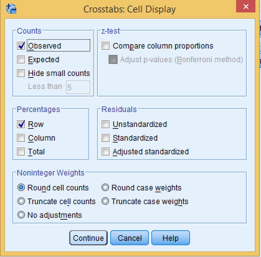
- Click Cells, tick Observed and Expected under Counts and Row under Percentages. Ticking Adjusted standardized under Residuals helps with tables larger than 2 × 2. Click Continue, then OK.
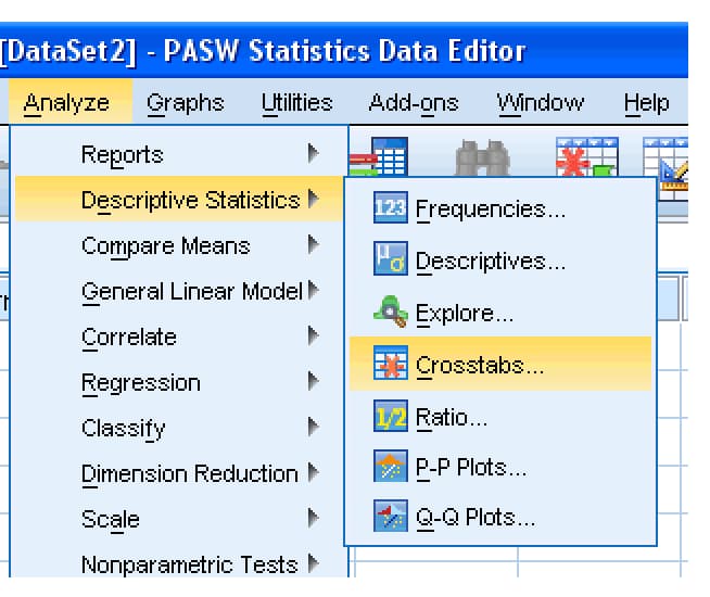
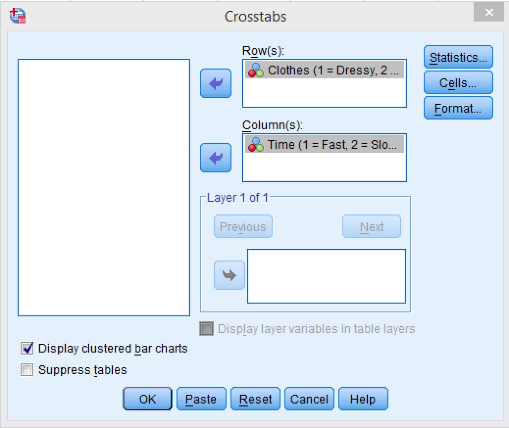
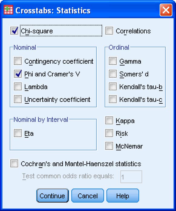
How to interpret chi-square output in SPSS
Skip the Case Processing Summary and read the remaining tables in order.
1. The crosstabulation
The table's title tells you exactly which variables you crossed. With row percentages, read across each row: 87.5% of dressy-condition salespeople were fast, compared with 37.5% in the sloppy condition. These percentages are what you describe in the write-up.
2. The Chi-Square Tests table
| Row | Value | When to use it |
|---|---|---|
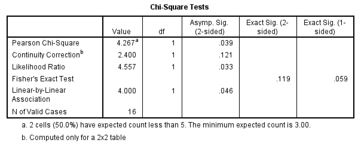
| Pearson Chi-Square | χ²(1) = 4.27, p = .039 | The standard result, when expected counts are adequate |
| Continuity Correction (Yates) | 2.40, p = .121 | A 2 × 2 adjustment; widely regarded as too conservative (Campbell, 2007) |
| Likelihood Ratio | 4.56, p = .033 | An alternative to Pearson's statistic, used in some fields |
| Fisher's Exact Test | p = .119 (two-sided) | 2 × 2 tables with small expected counts |
| Linear-by-Linear Association | 4.00, p = .046 | Only for ordered categories; ignore it for nominal variables |
Now the footnote: 2 cells (50.0%) have expected count less than 5. The minimum expected count is 3.00. This 2 × 2 table breaks the expected-count guideline, so the Pearson p value of .039 is not trustworthy, and the conventional choice is Fisher's exact test, p = .119, which is not significant (Kim, 2017). With only 16 salespeople, the data point in the predicted direction but do not provide clear evidence that clothing changed the speed of service.
Statisticians do not all agree on the best small-sample test. Campbell (2007) found that an "N − 1" version of the chi-square test is more accurate than Fisher's test for 2 × 2 tables when every expected count is at least 1; here it gives χ²(1) = 4.00, p = .046. When reasonable methods disagree like this, the honest conclusion is that the evidence is weak and a larger sample is needed. Follow the method your course or journal specifies, and decide on it before you see the results.
3. Symmetric Measures (effect size)
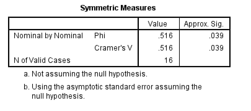
Phi (φ) is the effect size for a 2 × 2 table, and Cramér's V extends it to larger tables; for a 2 × 2 table, they are identical. Both run from 0 (no association) to 1. Cohen's (1992) benchmarks for this kind of effect are .10 small, .30 medium, and .50 large, so φ = .52 is large. With only 16 cases, though, the estimate is very imprecise, which is exactly why a large-looking effect can still fail to reach significance on an exact test. Convert between effect sizes with our effect size calculator.
Chi-square degrees of freedom
For a test of independence, df = (number of rows − 1) × (number of columns − 1). A 2 × 2 table has (2 − 1) × (2 − 1) = 1 df. Add a third clothing condition and the table becomes 3 × 2, so df = (3 − 1) × (2 − 1) = 2. For a goodness-of-fit test, df is the number of categories minus 1.
The degrees of freedom tell you how many cell counts are free to vary once the row and column totals are fixed. In a 2 × 2 table, once you know one cell and the totals, the other three are determined, so there is only one degree of freedom.
Chi-square for larger tables: three groups
Suppose the study adds a third group of customers in casual clothes, again with eight salespeople. The SPSS steps are the same; the table is now 3 × 2.
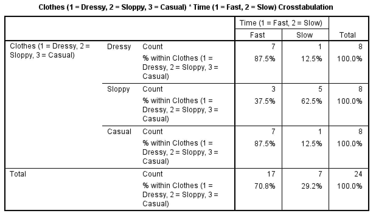
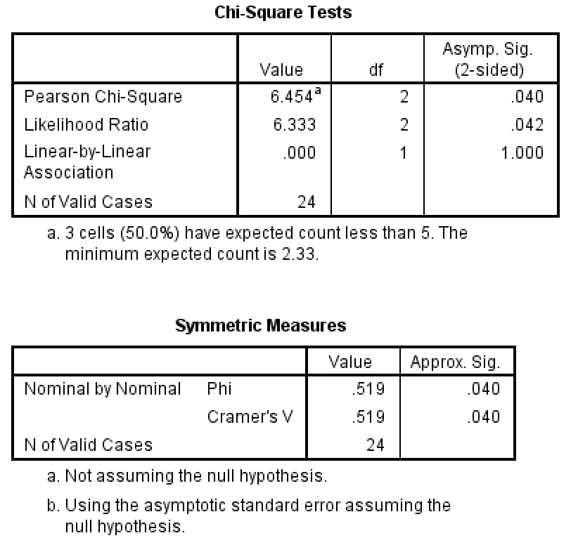
Pearson's test gives χ²(2, N = 24) = 6.45, p = .040, Cramér's V = .52. The footnote again warns that 3 of the 6 cells (50%) have expected counts below 5, well over the 20% guideline, and Fisher's test is not printed for tables larger than 2 × 2. An exact test of the whole table gives p = .062, so the same caution applies as before.
Which groups differ? Adjusted standardized residuals
A significant chi-square on a table larger than 2 × 2 tells you the variables are related, not which cells drive the relationship. Tick Adjusted standardized residuals in the Cells dialog: values beyond ±1.96 mark cells with more or fewer cases than expected at the .05 level (Field, 2024). Here, the sloppy condition has adjusted residuals of ±2.54 (more slow and fewer fast responses than expected), while dressy and casual are within ±1.27. So the sloppy group is the one that stands out.
How to report a chi-square test in APA 7
Report the test, the degrees of freedom and sample size in brackets, the value of χ², the exact p-value, an effect size, and the counts or percentages that show the direction of the relationship (American Psychological Association, 2020; Appelbaum et al., 2018). See our guide to reporting statistics in APA 7 for general formatting rules.
A chi-square test of independence examined the relationship between customers' clothing and how quickly salespeople approached them. Because two cells had expected counts below 5, Fisher's exact test was used. Salespeople approached 87.5% of customers in dressy clothes quickly, compared with 37.5% of customers in sloppy clothes, but the association was not statistically significant, p = .119 (Fisher's exact test, two-sided), φ = .52.
A chi-square test of independence showed a significant association between condition and willingness to volunteer, χ²(1, N = 120) = 9.70, p = .002, φ = .28. Participants in the experimental condition were more likely to volunteer (60.0%) than those in the control condition (31.7%).
Report non-significant results in the same format, for example χ²(1, N = 80) = 1.27, p = .260, φ = .13. Always give the actual p value rather than "p > .05", and present a table of counts and percentages when there are more than four cells.
Chi-square vs Fisher's exact test, t-test and ANOVA
| Test | Outcome variable | Use it when |
|---|---|---|
| Chi-square test of independence | Categorical | Two categorical variables and adequate expected counts |
| Fisher's exact test | Categorical | A 2 × 2 table with small expected counts |
| McNemar test | Categorical (paired) | The same people are classified twice, for example, before and after |
| Independent-samples t-test | Continuous | Comparing the means of two groups |
| One-way ANOVA | Continuous | Comparing the means of three or more groups |
The example in this guide turned approach times into fast and slow categories to demonstrate the chi-square test. With real data, you would normally keep the times in seconds and compare the groups with a t-test or a one-way ANOVA: splitting a continuous measure into categories throws information away and reduces power. Our guide to choosing a statistical test covers the full range of options.
Common chi-square mistakes
- Ignoring the expected-count footnote and reporting the Pearson result when Fisher's exact test is needed.
- Entering percentages instead of counts. The test needs raw frequencies.
- Counting the same person more than once, which breaks the independence assumption.
- Reporting the Linear-by-Linear Association row for nominal variables.
- Leaving out the direction. χ² says the variables are related; the percentages say how.
- Writing p = .000. Report p < .001.
- Splitting a continuous outcome into categories without a good reason, when a t-test or ANOVA on the original scores would be more powerful.
Getting help with chi-square in your statistics course
If you would like a specialist to check your SPSS setup, explain your output or give feedback on your APA results section, see our psychology research methods and statistics support. We explain each step so you can apply it confidently in your own work.
Frequently asked questions
What is a chi-square test of independence used for?
It tests whether two categorical variables are related, for example whether a juror's gender is associated with their verdict, by comparing observed counts with the counts expected if the variables were unrelated.
What is the difference between chi-square goodness of fit and test of independence?
A goodness-of-fit test uses one categorical variable and checks whether its counts match an expected distribution. A test of independence uses two categorical variables and checks whether they are related.
What do I do if an expected count is less than 5 in SPSS?
For a 2 × 2 table, report Fisher's exact test, which SPSS prints in the Chi-Square Tests table. For larger tables, use an exact test if available, combine categories where it makes sense, or collect more data.
When should I use Fisher's exact test instead of chi-square?
Use Fisher's exact test for 2 × 2 tables when any expected count is below 5, which usually happens with small samples.
How do I report a chi-square test in APA 7?
Write χ²(df, N = sample size) = value, p = value, followed by an effect size such as phi or Cramér's V and the percentages in each group, for example χ²(1, N = 120) = 9.70, p = .002, φ = .28.
How do you calculate degrees of freedom for a chi-square test?
For a test of independence, df = (rows − 1) × (columns − 1), so a 2 × 2 table has 1 df and a 3 × 2 table has 2. For goodness of fit, df is the number of categories minus 1.
How do I interpret Cramér's V and phi?
Both range from 0 to 1. Using Cohen's benchmarks, about .10 is small, .30 medium and .50 large. Phi is used for 2 × 2 tables; Cramér's V for larger tables.
Can I use a chi-square test instead of a t-test?
Only if your outcome is categorical. If it is a continuous score, use a t-test or ANOVA; turning scores into categories loses information.
Sources
- Field A. Discovering Statistics Using IBM SPSS Statistics. 6th ed. London: Sage; 2024
- Kim HY. Statistical notes for clinical researchers: chi-squared test and Fisher's exact test. Restor Dent Endod 2017;42(2):152-155
- Campbell I. Chi-squared and Fisher-Irwin tests of two-by-two tables with small sample recommendations. Stat Med 2007;26(19):3661-3675
- American Psychological Association. Publication Manual of the American Psychological Association. 7th ed. Washington, DC: American Psychological Association; 2020
- Appelbaum M, Cooper H, Kline RB, et al. Journal article reporting standards for quantitative research in psychology: the APA Publications and Communications Board task force report. Am Psychol 2018;73:3-25
- McHugh ML. The chi-square test of independence. Biochem Med (Zagreb) 2013;23(2):143-149
- Cohen J. A power primer. Psychol Bull 1992;112(1):155-159
- Cochran WG. Some methods for strengthening the common χ² tests. Biometrics 1954;10(4):417-451
- Smith RA, Davis SF. The Psychologist as Detective: An Introduction to Conducting Research in Psychology. Updated ed. Boston, MA: Pearson; 2016

Keith has 17 years of experience in experimental psychology and cognitive and behavioral research. He brings an experimental research perspective to projects that examine cognition, perception, and behavior. Areas of expertise Experimental and behavioral studies Quantitative research projects and data analysis…