
In a 2 × 2 factorial ANOVA, a main effect is the overall effect of one independent variable, averaged across the levels of the other: you compare its two marginal means. An interaction effect means the effect of one independent variable depends on the level of the other, so the difference between conditions is not the same at each level (a "difference in differences"). The ANOVA gives three F tests: one for each main effect and one for the A × B interaction. On a graph, parallel lines suggest no interaction and non-parallel lines suggest one. When the interaction is significant, the main effects are qualified by it, and you follow up with simple effects tests: the effect of one factor at each level of the other.
Working on a psychology methods assignment or lab report? Get one-to-one support from a specialist. Get a free quote →
What is a 2 × 2 factorial design?
A factorial design studies two or more independent variables (called factors) at the same time, with every level of one factor combined with every level of the other. The name gives the structure: in a 2 × 2 design there are two factors, each with two levels, which makes four conditions. A 2 × 3 design has two factors with two and three levels (six conditions), and a 2 × 2 × 2 design has three factors (eight conditions).
The analysis is called a two-way ANOVA, and you will also see it described as a factorial ANOVA, a univariate ANOVA (the name of the SPSS procedure) or a between-subjects ANOVA when each participant is in only one condition. Like a one-way ANOVA, it needs a continuous dependent variable, such as a rating scale or a time in seconds, and categorical independent variables (Field, 2024). A clear operational definition of each variable tells readers exactly what the factors and the outcome were.
The big advantage over running two separate one-way studies is that a factorial design answers three questions at once:
- Main effect of A: does factor A make a difference, averaging over B?
- Main effect of B: does factor B make a difference, averaging over A?
- A × B interaction: does the effect of A change depending on the level of B?
Each question has its own F test, so a two-way ANOVA always reports three F tests, plus up to four simple effects tests if the interaction is significant.
Main effect vs interaction effect
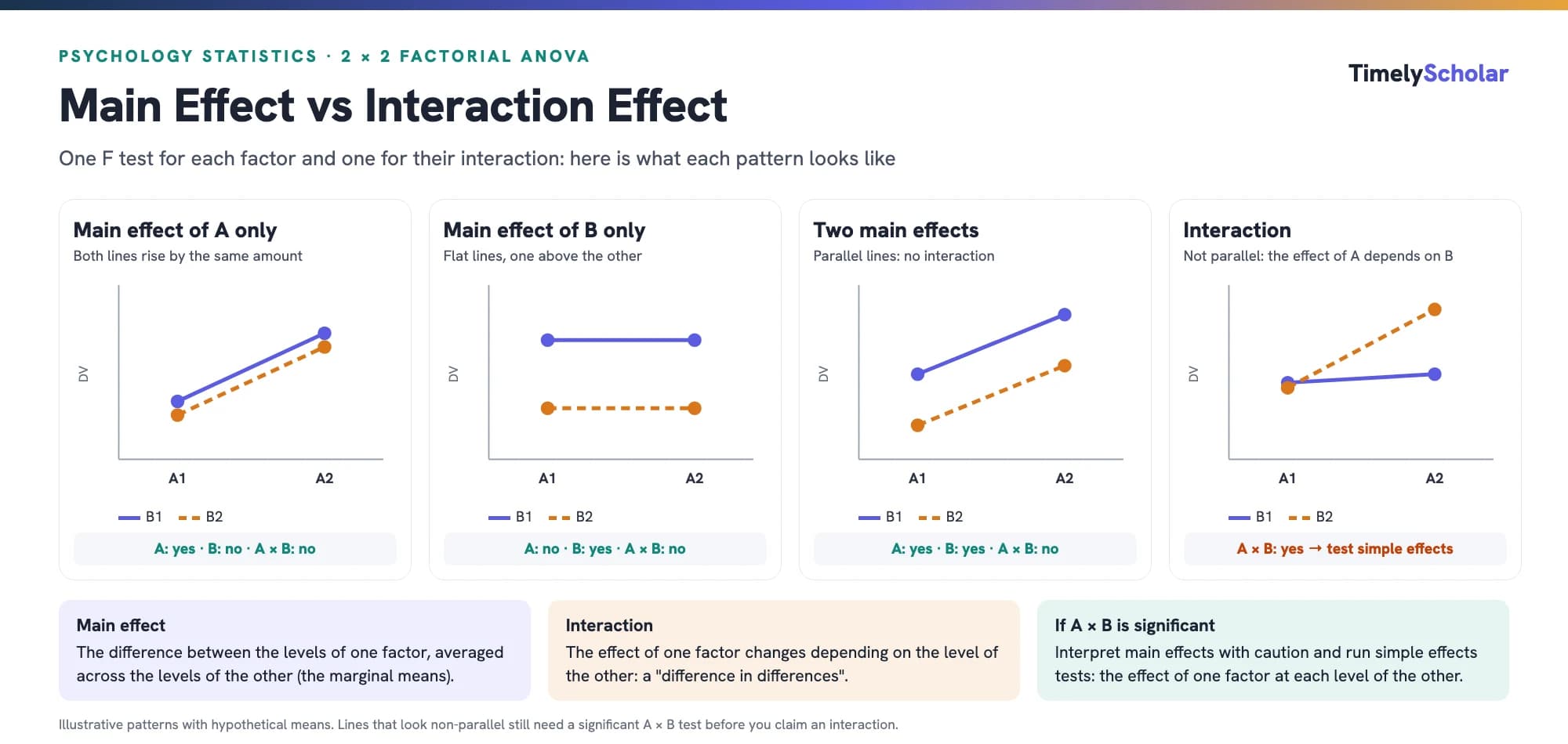
Main effect
A main effect is the difference between the levels of one factor averaged across the levels of the other. In a 2 × 2 design, each main effect compares just two numbers, the marginal means: the row or column averages of the four cell means. Because only two means are involved, a significant main effect needs no post hoc test; you simply look at which mean is higher.
Interaction effect
An interaction means the two factors combine in a way you could not predict from the main effects alone: the effect of one factor is different at different levels of the other. A useful way to think of it is as a difference in differences. Work out the effect of A at the first level of B, then at the second level of B. If those two differences are clearly unequal, there is an interaction. With four cell means instead of two, a significant interaction does not tell you which cells differ, which is why it needs follow-up tests.
| Main effect | Interaction (A × B) | |
|---|---|---|
| Question | Does one factor matter, on average? | Does the effect of one factor depend on the other? |
| Means compared | Two marginal means | All four cell means |
| On a line graph | Lines are higher or lower overall, or slope the same way | Lines are not parallel, or they cross |
| If significant | Compare the two means directly | Run simple effects tests |
Rohrer and Arslan (2021) add a further caution: an interaction is a vague claim unless you state what pattern you expect, because the same data can show an interaction on one scale of measurement and not on another (for example, raw seconds versus log-transformed times). Write down the specific pattern you predict, such as "clothing slows approach times for men but not for women", before you analyse the data.
Worked example: clothing × customer gender
The example below follows a classic textbook study (Smith & Davis, 2016). Salespeople were randomly assigned to see one of four customers, and the researchers timed, in seconds, how long it took them to approach the customer. The two factors are clothing (casual vs. sloppy) and customer gender (women vs. men), giving four conditions with six salespeople in each (N = 24). The dependent variable is the time to help, so higher numbers mean slower service.
| Customer | Casual clothes | Sloppy clothes | Marginal mean (gender) |
|---|---|---|---|
| Women | M = 48.17 (SD = 5.31) | M = 51.50 (SD = 12.21) | M = 49.83 (SD = 9.14) |
| Men | M = 45.67 (SD = 6.89) | M = 68.67 (SD = 11.15) | M = 57.17 (SD = 14.91) |
| Marginal mean (clothing) | M = 46.92 (SD = 6.01) | M = 60.08 (SD = 14.31) | M = 53.50 (SD = 12.66) |
Before running anything, read the table the way the ANOVA will (our guide to descriptive statistics explains cell means, marginal means and standard deviations):
- Clothing main effect: compare the bottom row. Casual customers were approached faster (46.92 s) than sloppy customers (60.08 s).
- Gender main effect: compare the right-hand column. Women were approached a little faster (49.83 s) than men (57.17 s).
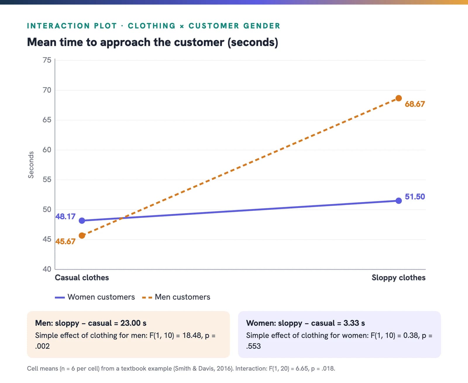
- Interaction: compare the effect of clothing for each gender. For women, sloppy clothes added 3.33 s (51.50 − 48.17); for men, they added 23.00 s (68.67 − 45.67). Those two differences are very unequal, which suggests an interaction.
How to run a two-way ANOVA in SPSS
Set up the data with one row per participant: a column for each factor (for example, Clothing: 1 = casual, 2 = sloppy; Gender: 1 = women, 2 = men) and a column for the dependent variable. Then:
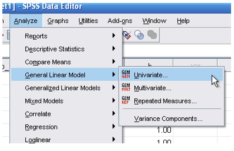
- Choose Analyze > General Linear Model > Univariate.
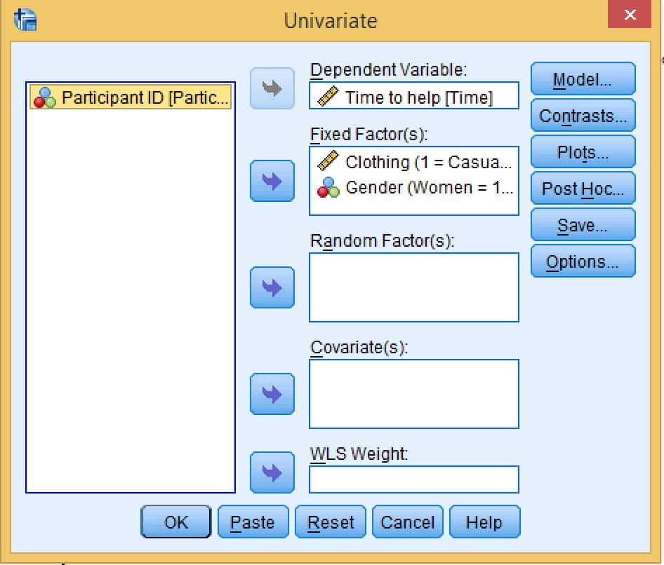
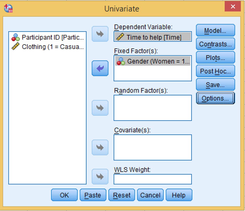
- Move the dependent variable (Time to help) into Dependent Variable and both factors into Fixed Factor(s).
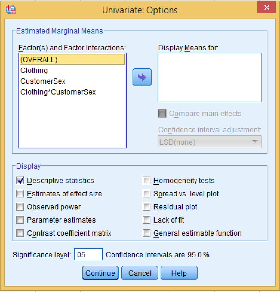
- Click Options, tick Descriptive statistics, and also tick Estimates of effect size and Homogeneity tests so you get partial eta squared and Levene's test. Click Continue, then OK.
Reading the output: main effects and the interaction
The Descriptive Statistics table gives the mean, standard deviation and n for each of the four cells and for each marginal total. These are the numbers you report alongside each F test. The bottom "Total, Total" row is the grand mean for all 24 participants, which you do not normally report.
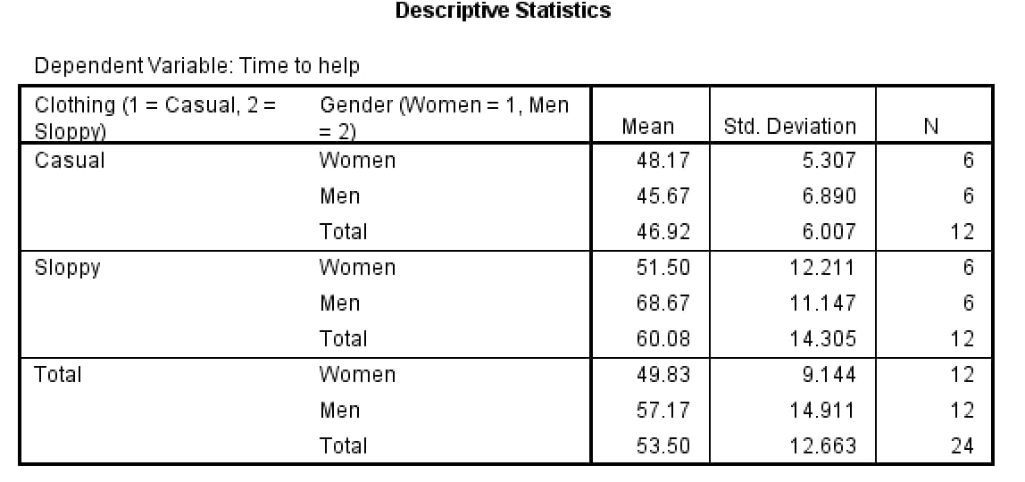
The ANOVA itself is in the Tests of Between-Subjects Effects table. Ignore the Corrected Model and Intercept rows and read the three rows named after your factors:
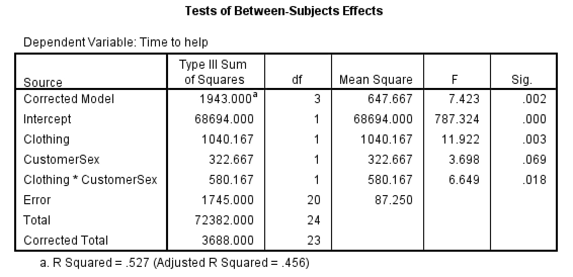
| Effect | F test | Partial η² | Result |
|---|---|---|---|
| Clothing (main effect) | F(1, 20) = 11.92, p = .003 | .37 | Significant |
| Customer gender (main effect) | F(1, 20) = 3.70, p = .069 | .16 | Not significant |
| Clothing × gender (interaction) | F(1, 20) = 6.65, p = .018 | .25 | Significant |
Each F has two degrees of freedom: the first comes from the effect's own row (1, because each factor has two levels) and the second from the Error row (20, which is N minus the four cells). Partial eta squared is the effect's sum of squares divided by the effect plus error sums of squares; it is the effect size SPSS reports for ANOVA, and reporting it lets readers compare results across studies (Lakens, 2013).
Why the main effects are "qualified"
Taken alone, the clothing main effect says sloppy customers wait longer. The interaction shows that this is true mainly for men: almost all of the 13-second clothing difference in the marginal means comes from the men's cells. When an interaction is significant, describe the main effects as qualified by the interaction and base your conclusions on the simple effects that follow (Field, 2024).
Simple effects tests: following up a significant interaction
A simple effect is the effect of one factor at one level of the other factor. In a 2 × 2 design there are four:
- Gender within casual clothing (casual women vs casual men).
- Gender within sloppy clothing (sloppy women vs sloppy men).
- Clothing within women (casual women vs sloppy women).
- Clothing within men (casual men vs sloppy men).
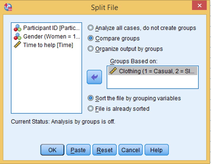
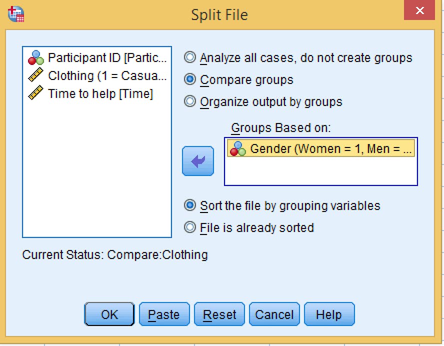
The simplest way to get them in SPSS is to split the file by one factor and rerun the ANOVA with only the other factor. SPSS then runs a separate analysis at each level of the split variable.
Effect of gender within each clothing condition
- Choose Data > Split File, select Compare groups, move Clothing into Groups Based on, and click OK.
- Rerun Analyze > General Linear Model > Univariate with Gender as the only fixed factor (remove Clothing), keeping Descriptive statistics ticked.
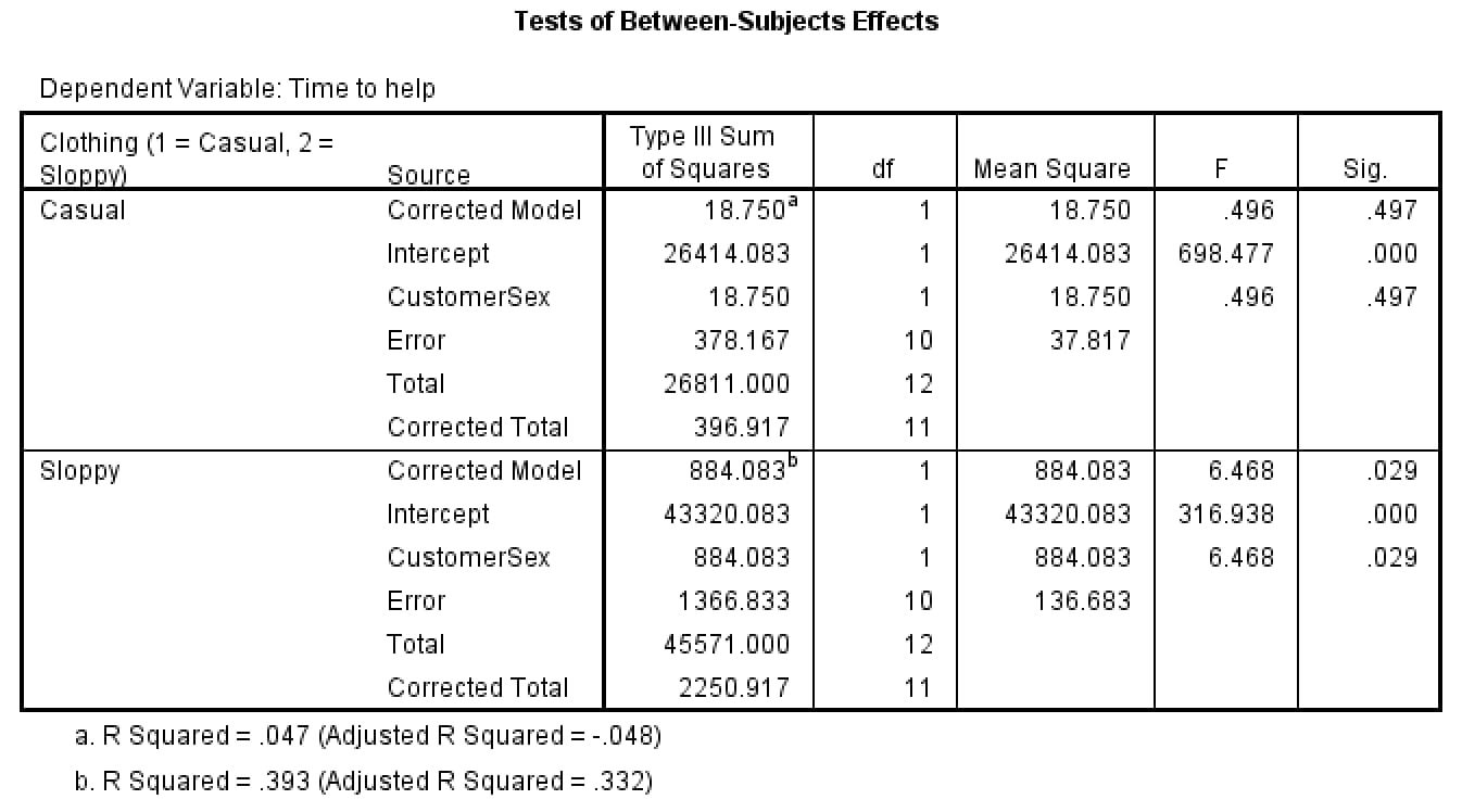
For casually dressed customers, gender made no difference, F(1, 10) = 0.50, p = .497. For sloppily dressed customers, salespeople approached women faster than men, F(1, 10) = 6.47, p = .029.
Effect of clothing for each gender
- Return to Data > Split File and replace Clothing with Gender in Groups Based on.
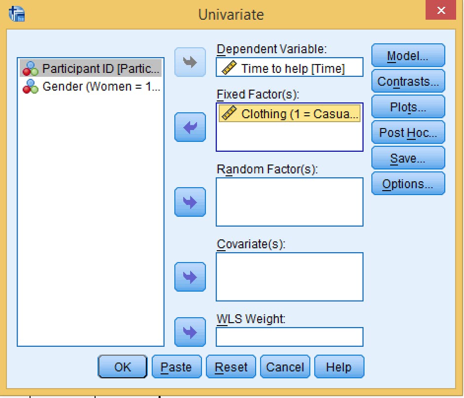
- Rerun the Univariate ANOVA with Clothing as the only fixed factor.
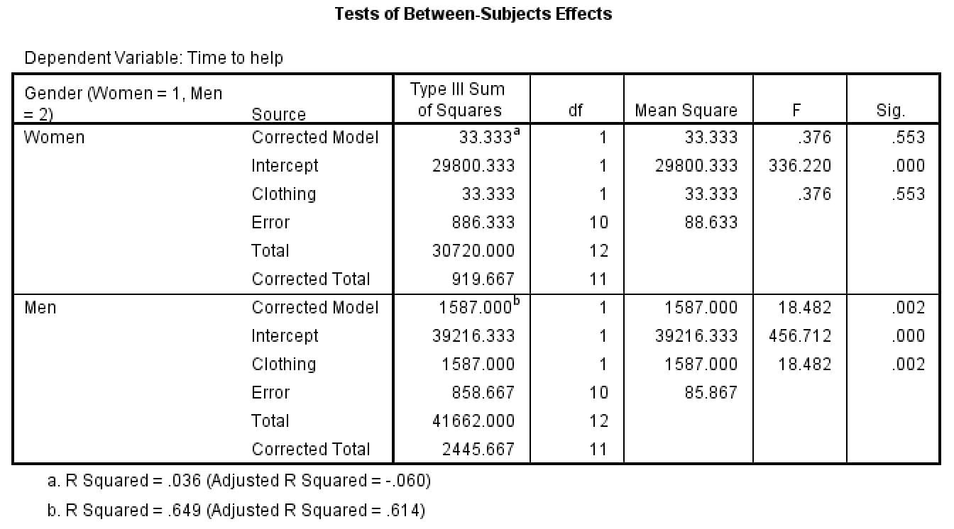
For women, clothing made no difference, F(1, 10) = 0.38, p = .553. For men, sloppy clothing slowed service considerably, F(1, 10) = 18.48, p = .002. Each of these simple effects compares just two means, so it is equivalent to an independent-samples t-test on those two cells (F = t²). Remember to switch the split off afterwards (Data > Split File > Analyze all cases) so later analyses use the whole sample.
Two refinements worth knowing
- Multiple tests. Four simple effects tests raise the chance of a false positive. A Bonferroni correction tests each at .05 / 4 = .0125. Here the clothing effect for men (p = .002) survives, but the gender difference in the sloppy condition (p = .029) would not. Follow your course's guidance on whether to correct.
- Pooled error term. Split-file tests use only the error variance from the cells being compared (df = 10). Many texts instead test simple effects against the error term from the full ANOVA (df = 20), which SPSS produces with an EMMEANS command with COMPARE and a Bonferroni adjustment in the GLM syntax (Field, 2024). With the pooled error, the gender difference for sloppy customers is F(1, 20) = 10.13, p = .005. The pooled approach has more power but assumes the cell variances are similar, so check Levene's test first.
Writing up a 2 × 2 ANOVA in APA style
Report each main effect, then the interaction, then the simple effects, giving F with both degrees of freedom, the exact p value and an effect size, with means and standard deviations either in the text or in a table (American Psychological Association, 2020; Appelbaum et al., 2018). Our guide to reporting statistics in APA 7 covers the formatting rules.
A 2 (clothing: casual, sloppy) × 2 (customer gender: women, men) between-subjects ANOVA was conducted on the time salespeople took to approach the customer. There was a significant main effect of clothing, F(1, 20) = 11.92, p = .003, η²ₚ = .37: casually dressed customers were approached faster (M = 46.92 s, SD = 6.01) than sloppily dressed customers (M = 60.08 s, SD = 14.31). The main effect of customer gender was not significant, F(1, 20) = 3.70, p = .069, η²ₚ = .16.
These effects were qualified by a significant clothing × gender interaction, F(1, 20) = 6.65, p = .018, η²ₚ = .25. Simple effects tests showed that clothing affected approach times for men, F(1, 10) = 18.48, p = .002, with sloppily dressed men approached more slowly (M = 68.67, SD = 11.15) than casually dressed men (M = 45.67, SD = 6.89), but not for women, F(1, 10) = 0.38, p = .553. Sloppily dressed women were approached faster than sloppily dressed men, F(1, 10) = 6.47, p = .029, whereas gender made no difference for casually dressed customers, F(1, 10) = 0.50, p = .497.
If the paragraph becomes crowded, put the cell and marginal means in a table and refer to it, keeping the F tests in the text. If the interaction is not significant, report it as such (for example F(1, 20) = 1.20, p = .286) and interpret the main effects directly; no simple effects tests are needed.
Assumptions and sample size
- Continuous dependent variable measured on an interval or ratio scale; categorical outcomes need a different test, such as chi-square.
- Independent observations: each participant contributes to one cell only. If the same people take part in every condition, use a repeated-measures or mixed ANOVA instead.
- Approximately normal residuals within each cell, which matters less as cell sizes grow.
- Similar variances across cells, checked with Levene's test. In the example, the standard deviations range from about 5 to 12 seconds, so this is worth checking and reporting.
Sample size deserves particular attention. Six participants per cell is fine for a textbook demonstration but far too small for a real study. Brysbaert (2019) shows that many psychology experiments are underpowered, and Sommet et al. (2023) demonstrate that detecting an interaction, especially one where an effect is weaker in one condition rather than reversed, usually requires many more participants than detecting a main effect of the same size. Run a power analysis for the interaction you predict before collecting data; our power analysis calculator is a quick starting point.
Common mistakes with main effects and interactions
- Interpreting a main effect at face value when the interaction is significant. Say the main effect is qualified, and draw conclusions from the simple effects.
- Comparing the four cell means by eye. A significant interaction does not tell you which cells differ; simple effects tests do.
- Reporting only p values. Include the F, both degrees of freedom, the effect size and the means.
- Forgetting to turn the split file off, so that later analyses run separately for each group.
- Calling a non-significant interaction "no difference between the conditions". It means the effect of one factor did not reliably change across the other, not that all four means are equal.
- Running a two-way ANOVA on a categorical outcome such as yes/no answers.
Getting help with your research methods course
Factorial ANOVA sits at the centre of most psychology statistics courses, and simple effects are where many students get stuck. If you would like a specialist to check your SPSS setup, talk through your output or give feedback on your APA results section, see our psychology research methods and statistics support. We explain each step so you can apply it yourself.
Frequently asked questions
What is the difference between a main effect and an interaction effect?
A main effect is the overall effect of one independent variable, averaged across the levels of the other. An interaction effect means the effect of one independent variable changes depending on the level of the other, so the difference between conditions is not the same at each level.
How many F tests are there in a 2 × 2 ANOVA?
Three: one for the main effect of each factor and one for the A × B interaction. If the interaction is significant, up to four simple effects tests follow.
How do you know if there is an interaction in a two-way ANOVA?
Look at the A × B row of the Tests of Between-Subjects Effects table in SPSS. If its p value is below .05, the interaction is significant. A line graph of the cell means helps you see it: non-parallel lines suggest an interaction.
What do you do when the interaction is significant?
Treat the main effects as qualified by the interaction and run simple effects tests: the effect of one factor at each level of the other. In SPSS you can split the file by one factor and rerun the ANOVA with the other factor, or use EMMEANS syntax with the pooled error term.
Can you have an interaction without main effects?
Yes. In a crossover interaction the effect of one factor reverses at the two levels of the other, so the marginal means can be equal and neither main effect is significant even though the interaction is.
What are simple effects tests?
They test the effect of one factor at a single level of the other factor, for example the effect of clothing for men only and for women only. They are the follow-up to a significant interaction, much as post hoc tests follow a significant one-way ANOVA.
How do I report a two-way ANOVA in APA style?
Report each main effect and the interaction as F(df effect, df error) = value, p = value, with an effect size such as partial eta squared, and give the means and standard deviations. If the interaction is significant, add the simple effects tests in the same format.
Sources
- Field A. Discovering Statistics Using IBM SPSS Statistics. 6th ed. London: Sage; 2024
- Sommet N, Weissman DL, Cheutin N, Elliot AJ. How many participants do I need to test an interaction? Conducting an appropriate power analysis and achieving sufficient power to detect an interaction. Adv Methods Pract Psychol Sci 2023;6(3)
- Rohrer JM, Arslan RC. Precise answers to vague questions: issues with interactions. Adv Methods Pract Psychol Sci 2021;4(2)
- American Psychological Association. Publication Manual of the American Psychological Association. 7th ed. Washington, DC: American Psychological Association; 2020
- Brysbaert M. How many participants do we have to include in properly powered experiments? A tutorial of power analysis with reference tables. J Cogn 2019;2(1):16
- Appelbaum M, Cooper H, Kline RB, et al. Journal article reporting standards for quantitative research in psychology: the APA Publications and Communications Board task force report. Am Psychol 2018;73:3-25
- Lakens D. Calculating and reporting effect sizes to facilitate cumulative science: a practical primer for t-tests and ANOVAs. Front Psychol 2013;4:863
- Smith RA, Davis SF. The Psychologist as Detective: An Introduction to Conducting Research in Psychology. Updated ed. Boston, MA: Pearson; 2016

Keith has 17 years of experience in experimental psychology and cognitive and behavioral research. He brings an experimental research perspective to projects that examine cognition, perception, and behavior. Areas of expertise Experimental and behavioral studies Quantitative research projects and data analysis…